🤗Introduction to Generative Models

Generative Models are part of unsupervised learning models that can learned from the datasets without any labels. Unlike other unsupervised models to manipulate, denoise, interpolate between, or compress examples, generative models focus on generating plausible new samples having similar properties to the dataset.

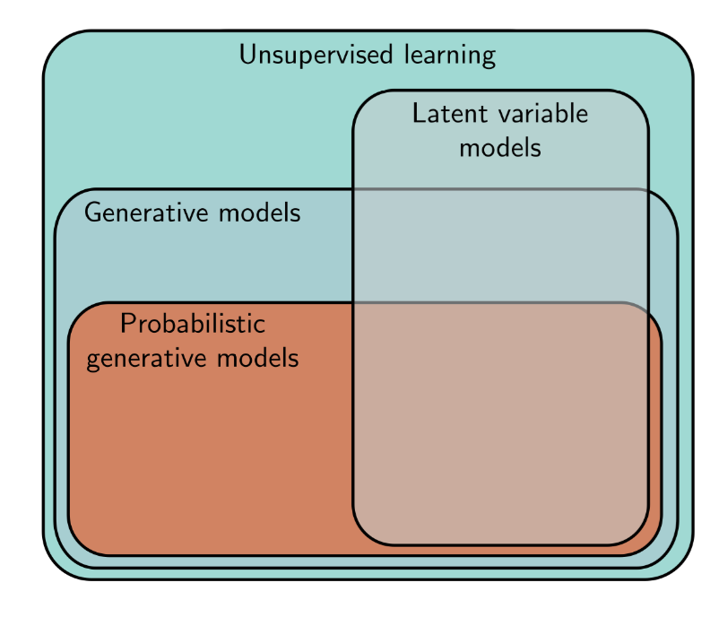
Taxonomy of unsupervised learning models

Latent variable models: mapping the data examples $\mathbf{x}$ to unseen latent variables $\mathbf{z}$ which can capture the underlying structure in the dataset.

In this essay, we will introduce the categories of generative models, discuss their properties, and talk about how to measure them.

What are probabilistic models?

Before we dive into the typical forms of generative models, we should understand two major categories of them.

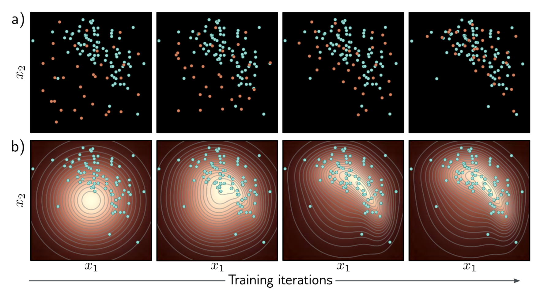
Direct generative models, such as generative adversarial models, aim to provide a mechanism for generating samples similar to observed data $\{\mathbf{x}_i\}$
Probabilistic models learn the probability distribution over the train data. These models will assign a probability $Pr(\mathbf{x}|\phi)$ to each data point $\mathbf{x}$. The models aim to maximize the probability of the observed data $\{\mathbf{x}_i\}$.
$$ L[\phi]=-\sum_{i=1}^{I}\mathrm{log}[Pr(\mathbf{x}_i|\phi)] $$

There is an image to describe the training process of the two models.

Properties of Generative Models

There are several properties that Generative Models need to have:

Efficient sampling: using less computational consumption.
High-quality sampling: output is indistinguishable from train data
Coverage: samples should represent the entire training distribution
Well-behaved latent space: change in latent space will perform in data similarly.
Efficient likelihood computation: able to calculate the probability of new examples efficiently.

It’s hard for only one type of Generative Model to obtain all properties, following is a table to describe some generative model’s features:

Model	Probabilistic	Efficient	Sample quality	Coverage	Well-behaved latent space	Disentangled latent space	Efficient likelihood
GANs	✖️	✔️	✔️	✖️	✔️	❔	\
Flows	✔️	✔️	✖️	❔	✔️	❔	✖️
VAEs	✔️	✔️	✖️	❔	✔️	❔	✔️
Diffusion	✔️	✖️	✔️	❔	✖️	✖️	✖️

Performance Measurement

To measure the performance of generative models, some metrics are proposed.

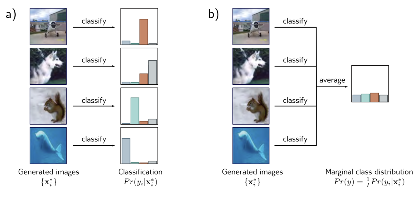
Inception score (IS): This metric is used in image generative models which trained on the ImageNet dataset. There are two criteria to design it. First, each generated image $\mathbf{x}^*$ should look like only one class in the ImageNet dataset which has 1000 possible classes. Second, the probability for each class in generated images should be equal.

This metric uses KL divergence between $Pr(y_i|\mathbf{x}_i^*)$and $Pr(y)$

$$ IS=\mathrm{exp}\bigg[\frac{1}{I}\sum_{i=1}^{I}D_{KL}\big[Pr(y_i|\mathbf{x}_i^*)||Pr(y)\big]\bigg] $$

Where $I$ is the number of generated images and:

$$ Pr(y)=\frac{1}{I}\sum_{i=1}^{I}Pr(y_i|\mathbf{x}_i^*) $$

Fréchet inception distance: To decrease the reliance on the ImageNet dataset and characterize either distribution, the Fréchet inception distance is estimated.

First, use the inception model accepting both observed and generated images as input to produce $1\times 2048$ feature vector. And, because the images follow the normal distribution which can be defined by mean and variance, we can use them to calculate the distance between real and generated images.

Above all, the formula for calculating FID can be written as follows:

$$ FID(x,g)=||\mu_x-\mu_g||_2^2+Tr\big(\Sigma_x+\Sigma_g-2(\Sigma_x\Sigma_g)^{0.5}\big) $$

Where $x,g$ present real and generated images, $\mu$ is the mean and $\Sigma$ is the covariance.

However, this metric uses the inception network output to calculate, which will more focus on the semantic information.

Manifold precision/recall: To disentangle the realism of the samples and their diversity, we consider the overlap between the data manifold and the model manifold.

Precision is the fraction of model samples that fall into the data manifold.
Recall is the fraction of data examples that fall within the model manifold.

Reference

[1] C. Szegedy, V. Vanhoucke, S. Ioffe, J. Shlens, and Z. Wojna, ‘Rethinking the Inception Architecture for Computer Vision’, in Proceedings of the IEEE Conference on Computer Vision and Pattern Recognition (CVPR), 2016.

[2] M. Heusel, H. Ramsauer, T. Unterthiner, B. Nessler, and S. Hochreiter, ‘GANs Trained by a Two Time-Scale Update Rule Converge to a Local Nash Equilibrium’, in Advances in Neural Information Processing Systems, 2017, vol. 30.

[3] S. J. D. Prince, Understanding Deep Learning. MIT Press, 2023.