📃Different Normalization
Introduction Link to heading
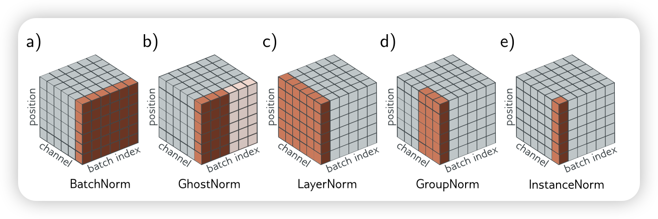
Normalization techniques are fundamental to training deep learning models effectively. They help stabilize and accelerate training, improve generalization, and prevent internal covariate shift. Below is a summary of the most common normalization techniques, their mechanisms, key papers, and differences.
🔑 Summary of different type of Normalization Link to heading
| Name | Normalized Over | Key Paper | Common Use Cases | Strength | Weakness |
|---|---|---|---|---|---|
| Batch Normalization (BN) | For Conv: per channel across B×H×W; For MLP: per feature across B. | Batch Normalization: Accelerating Deep Network Training by Reducing Internal Covariate Shift (ICML 2015) | Computer Vision Field like Image Classification, Detection, Segmentation | Stabilizes activation scale; Enables larger learning rates, Speeds convergence; Adds implicit regularization | Less suited to online / streaming / RNN small-batch settings, can cause issues in domain shift or micro-batch training |
| Layer Normalization (LN) | Per sample (token) across its feature (hidden) dimensions (e.g. For shape B×L×D or B×D: normalize over D; for Conv rarely used, would be over C×H×W of that sample) | Layer Normalization (arXiv 2016) | Transformers (NLP & Vision), RNNs, small-batch or batch=1 training | Independent of batch size, identical behavior in training & inference, stable for variable-length sequences, improves gradient flow (esp. Pre-LN Transformers) | Provides less implicit regularization, does not leverage cross-sample statistics |
| Instance Normalization (IN) | For conv input BxCxHxW: each sample & channel independently over its spatial pixels HxW (no cross-batch, no cross-channel). | Instance Normalization: The Missing Ingredient for Fast Stylization (ECCV 2016) | image generation (GAN generators), image-to-image translation (e.g., style/appearance adaptation) | Batch size–independent, effectively strips instance-specific style (contrast, color cast), aiding fast stylization | Discards global intensity/contrast cues useful for recognition → poorer performance on classification/detection; lacks batch-level regularization |
| Group Normalization (GN) | For input BxCxHxW: per sample, split channels into G groups (size C/G); compute mean & var over (C/G)xHxW inside each group. | Group Normalization (ECCV 2018) | Small-/micro-batch CNN training, cases where BN fails with batch sizes 1–4. | Batch-size independent; stable for tiny or variable batches; often better than BN when batch is very small. | Extra hyperparameter (G) to tune; less implicit regularization than BN, grouping may not align with the semantic channel structure |
| Weight Normalization (WN) | Each weight vector of a neuron/output channel. | Weight Normalization: A Simple Reparameterization to Accelerate Training of Deep Neural Networks (NIPS 2016) | RNN / seq models where BN is hard, small-batch or online / RL training (policy & value nets) | Negligible inference cost (can fold into static weights); works with streaming / RL; complements other norms (can combine with LayerNorm) | Scale may drift (need LR tuning); benefit can vanish with strong adaptive optimizers; less helpful for very deep Transformers (other norms preferred) |
| Spectral Normalization (SN) | Each weight tensor (e.g. matrix / conv kernel reshaped to 2D) | Spectral Normalization for Generative Adversarial Networks (ICLR 2018) | GAN discriminators, robustness / Lipschitz-constrained models, etc. | Enforces (approx.) 1-Lipschitz per layer (controls gradient explosion) | Extra cost (power iteration each step); only constrains the largest singular value (other singular values can still drift) |
| RMS Normalization | Per sample (token) feature vector | Root Mean Square Layer Normalization (NIPS 2019) | Modern Transformer / LLM blocks; very deep pre-norm architectures, low-precision (FP16/BF16) | Simpler & slightly cheaper than LayerNorm, numerically stable in mixed precision, good for very deep stacks (retains strong gradient path) | Mean not zeroer, possible drift, needs careful init/residual scaling, and isn’t fully interchangeable with zero-mean LN methods. |
📘 Explanation of How They Work Link to heading
Batch Normalization (BN) Link to heading
The Batch Normalization normally used in computer vision field, typically the CNN. Generally, the input shape of BN is $\text{Batch}(B)\times \text{Channel}(C) \times \text{Height}(H)\times\text{Width}(W)$.
Calculate progress: Compute mean & variance across the batch and apply learnable scale $\gamma$ and shift $\beta$:
$$ \mu_c=\frac{1}{B\cdot H\cdot W}\sum_{i=1}^B \sum_{j=1}^H\sum_{k=1}^Wx_{i,c,j,k} $$$$ \sigma_c^2=\frac{1}{B\cdot H\cdot W}\sum_{i=1}^B \sum_{j=1}^H\sum_{k=1}^W(x_{i,c,j,k}-\mu_c)^2 $$$$ \hat{x}_{c} = \frac{x_c - \mu_c}{\sqrt{\sigma^2_c + \epsilon}} $$$$ y_c = \gamma_c \hat{x}_c + \beta_c $$-
Why separate the Channel dimension during calculating the $\mu, \sigma$?
The Channel usually represent the different feature of the sample, such as color, texture, which shouldn’t be normalized together.
-
Why cross different sample in the batch?
- Using $B\times H\times W$ numbers gives a smoother (less noisy) mean and variance.
- Remove sample-level shift.
- Add noice between different batch as regulation
Layer Normalization (LN) Link to heading
The Layer Normalization normally used in NLP field. Generally, the input shape will look like $\text{Batch}(B)\times \text{Length}(L) \times \text{Token}(D)$.
$$ \mu_{b,l} = \frac{1}{D}\sum_{d=1}^{D} x_{b,l,d} $$$$ \sigma_{b,l}^{2} = \frac{1}{D}\sum_{d=1}^{D} (x_{b,l,d}-\mu_{b,l})^{2} $$$$ \hat{x}_{b,l} = \frac{x_{b,l}-\mu_{b,l}}{\sqrt{\sigma_{b,l}^2+\varepsilon}} $$$$ y_{b,l} = \gamma_{d}\,\hat{x}_{b,l} + \beta_{d} $$-
Why not treat the sequence length L as part of the feature dimension?
Because in NLP the feature (channel) dimension is in the hidden size $D$; positions along L are different tokens, not different feature subspaces of the same token. Channels describe aspects of one token; sequence positions index different tokens. Mixing over $L$ would entangle token-specific information.
-
Why use Pre-LN?
Pre-LN moved LN before each sublayer so that residual additions remain pure identity shortcuts, dramatically improving gradient flow and training stability—critical for very deep or large Transformers—at the cost of needing a final normalization and sometimes explicit residual scaling to control activation growth.
Instance Normalization (IN) Link to heading
Normally use in Computer Vision, Generally, the input shape of BN is $\text{Batch}(B)\times \text{Channel}(C) \times \text{Height}(H)\times\text{Width}(W)$.
$$ \mu_{b,c}=\frac{1}{H\cdot W}\sum_{j=1}^H\sum_{k=1}^Wx_{b,c,j,k} $$$$ \sigma_{b,c}^2=\frac{1}{H\cdot W} \sum_{j=1}^H\sum_{k=1}^W(x_{b,c,j,k}-\mu_{b,c})^2 $$$$ \hat{x}_{b,l} = \frac{x_{b,l}-\mu_{b,l}}{\sqrt{\sigma^{2}_{b,l}+\varepsilon}} $$$$ y_{b,} = \gamma_{d}\,\hat{x}_{b,l} + \beta_{d} $$-
What different Between Layer Normalization and Instance Normalization?
Also they look like both deal with the last channel, but actually LayerNorm (LN) normalizes the entire feature vector / channel set of a single sample together; InstanceNorm (IN) normalizes each channel’s spatial dimensions of the same sample separately (without mixing channels).
Group Normalization (GN) Link to heading
The Group Normalization widely used in CV when batch-size is lower. This method Divide channels into G groups, normalize each group.
$$ \mu_{bg}=\frac{1}{(C/G)\cdot H\cdot W}\sum_{i=g(C/G)}^{(g+1)(C/G)} \sum_{j=1}^H\sum_{k=1}^Wx_{b,i,j,k} $$$$ \sigma_{bg}^2=\frac{1}{(C/G)\cdot H\cdot W}\sum_{i=g(C/G)}^{(g+1)(C/G)} \sum_{j=1}^H\sum_{k=1}^W(x_{b,i,j,k}-\mu_{bg})^2 $$$$ \hat{x}_{bg} = \frac{x_{bg} - \mu_{bg}}{\sqrt{\sigma^2_{bg} + \epsilon}} $$$$ \ y_{bg} = \gamma_{bg} \hat{x}_{bg} + \beta_{bg} $$Flexible continuum between LN (G=1) and IN (G=C);
Weight Normalization (WN) Link to heading
Re-parameterizes weights as:
$$ \mathbf{x}=\frac{g}{||\mathbf{v}|| }\cdot\mathbf{v} $$- $g$ is a learnable scalar.
- $\mathbf{v}$ is a direction vector
Advantage:
- More convenient for gradient update
- Adapt with Dropout, BN, etc.
Spectral Normalization (SN) Link to heading
Spectral Normalization is a technique that normalizes the weights of a neural network layer by dividing them by their spectral norm (i.e., the largest singular value of the weight matrix).
$$ ||\mathbf{W}||_2=\sigma_{\text{MAX}}(\mathbf{W})\\\hat{\mathbf{W}}=\frac{\mathbf{W}}{||\mathbf{W}||_2} $$RMS Normalization Link to heading
Variant of LayerNorm that uses RMS (root mean square) instead of mean & variance, removing the mean normalization step.
$$ \text{RMS}(x)=\sqrt{\frac{1}{d}\sum_{i=1}^{d}x_i^2+\epsilon} $$$$ \text{RMSNorm(x)}=\frac{x}{\text{RMS}(x)}\cdot \gamma $$📝 Summary Link to heading
This post is a quick field guide to seven of the most widely used normalization methods in deep learning—BatchNorm, LayerNorm, InstanceNorm, GroupNorm, WeightNorm, Spectral Norm, and RMS Norm. For each, it explains what is being normalized, how it’s computed (with key formulas), where it first appeared, and the typical scenarios in which it shines or struggles. By contrasting their underlying statistics (batch-level vs. sample-level, feature-wise vs. weight-wise) and listing practical pros / cons, the blog equips researchers and practitioners to choose the right normalizer for everything from tiny-batch CNNs to giant Transformer stacks, GANs, and reinforcement-learning agents.